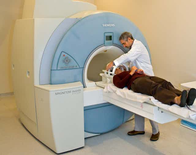

Our short series, the Science of Medical Imaging, examines the technology behind non-invasive methods of creating images of the human body. In this third and final instalment, we look at the basics of magnetic resonance imaging (MRI).
In the first two articles in this series we saw that emission imaging provides functional information and transmission imaging provides structural context in the body.
The previously-discussed techniques are hugely beneficial; however, their repeated use on a given patient must be limited as they utilise ionising radiation.
In the context of this discussion, it is important to remember that we are exposed to ionising radiation every day and our bodies do an excellent job in ameliorating any effects.
It remains true, though, that exposure to ionising radiation even as a part of effective clinical care can have a negative effect. One key technique that circumvents some of these issues is magnetic resonance imaging (MRI).
Mapping water
MRI was first used for imaging in the 1970s and since then, has seen many improvements. One of these, functional MRI (fMRI), allows changes in neuronal function to be observed while the patient performs a task.
MRI most commonly maps the distribution of water in the body. Water is composed of two hydrogen atoms and a single oxygen atom.
We can imagine these two hydrogens at the end of oxygen’s two “arms”. It is this specific molecular shape that allows MRI to pick out the hydrogens within water molecules.
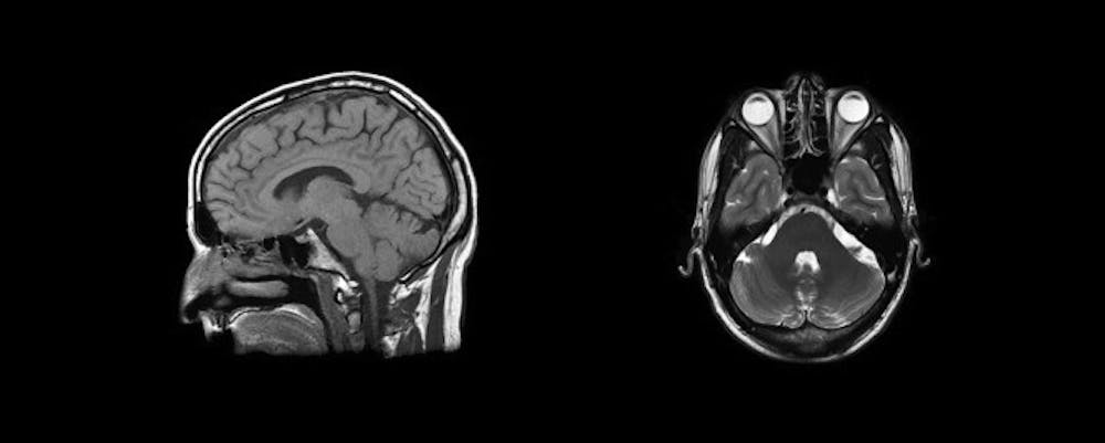
Your brain and other soft tissue are 60-70% water compared to your bones which are only 30% water, so MRI is much better at mapping soft tissue. As you can see in the MRI image below, the aqueous humour of the eye shows up white, while skull bones are comparatively dark.
Generating magnetic resonance
A complete description of MRI requires an understanding of quantum mechanics and spin, but in the interests of article brevity, let’s ignore them.
All we really need to note is that we rely on protons acting as magnetic dipoles. Simply put, a dipole is an object with two opposing poles. Thus, a magnetic dipole - such as a bar magnet - has north and south magnetic poles.
The orientation of the bar magnet in space can be described by the magnetic dipole moment which is a vector (as it has a direction, being from the south to the north pole).
The nucleus of the hydrogen atom in water has just one proton and it is the magnetic property of the proton that generates the signal in MRI.
To understand magnetic resonance, first start by making the assumption that the dipole moment of a single proton in a uniform magnetic field behaves like a compass needle.
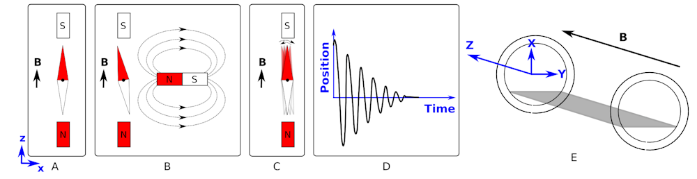
Figure A shows that a compass needle placed in a magnetic field aligns with the field. The direction of the field is indicated by the vector B in the diagram.
We can then “kick” (excite) the system by introducing a second magnetic field (figure B) and then subsequently removing it (figure C). This will cause the needle to rock back and forth like a pendulum until it returns to its rest position.
If we plotted the position of the red part of the needle relative to its start position, we would get something like the shape shown in figure D.
This shape of graph is called a damped sinusoidal wave. It is given this name as oscillates like a cosine (or sine) wave but its magnitude decreases (is damped) with time.
If, instead of removing the magnet entirely, we slide the second magnet back and forth (along the x-axis) at the correct frequency, we give the maximum “kick” to the needle and achieve a resonance.
This is analogous to choosing the correct times at which you push a child on a swing to gain maximum height.
Now, back to a practical discussion of MRI. Imagine a patient is laying in the scanner along the z-axis (see figure E) - the same direction as the strong magnetic field. We have already demonstrated what happens if the protons in the water in your body behaved like compass needles (see figure A) - they align with the magnetic field.
However, because the protons have spin (angular momentum), they can align along or at 180 degrees to the field. These are two different energy states. There is not an exact 50:50 split and slightly more (an excess) of the protons align in the same direction as the magnetic field.
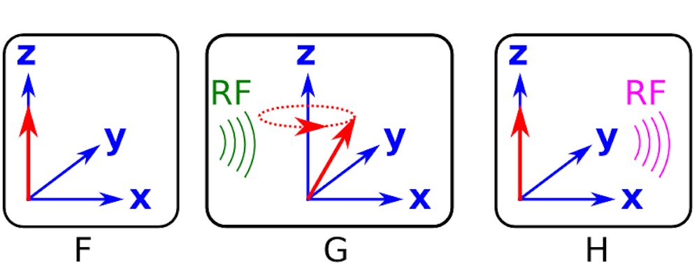
Figure F shows a cartoon of the excess of aligned protons (red arrows) in the patient. They appear as only a single red arrow because the dipole moment for each proton is sat on top of all the others.
Now, we need to “kick” the system. The way we do this is not with a bar magnet (as in figures B and C), but with a suitable radio frequency signal, approximately 60 MHz.
A radio frequency wave has both electric and magnetic fields. By generating a radio frequency wave and passing it through the body we disturb the protons, giving them energy. The protons have spin and so they precess around the z-axis (as opposed to just rocking back and forth like the compass needle).
An example of the protons precessing after the radio frequency wave has “kicked” the system is shown in figure G. The frequency of this precession is proportional to the strength of the magnetic field and is called the Larmor frequency. Again, in figure G, all of the protons are precessing at the same frequency and so the arrows are sat on top of one and other.
Up until now, all we have done is prepare the system by putting in energy in terms of electromagnetic fields - we haven’t actually measured anything. After the radio frequency pulse is applied, the precessing protons return to their equilibrium positions by emitting radio frequency waves (see figure H).
It is the magnetic field of this radio frequency wave - the magnetic resonance - that provides us with a signal that we can measure, and we do so with an induction coil.
Like we showed for the compass, the signal measured in magnetic resonance is also a damped sinusoidal wave that is caused by the dipole moments returning to their original orientations.
The signal shape is determined by the precession frequency and another effect called dephasing (see the second definition on this Wikipedia page). The dephasing causes the dipole moments of the protons to separate out rather than sitting on top of each other as is shown in figures F to H.
Locating the signal
There is still a problem as we have not mentioned anything about determining where in the patient the signal comes from. After all, if we want to produce a map of the distribution of proton density in the patient (the image), we need to know the position of the emission of the radio frequency wave.
When we look at the signals, they have two main properties of interest:
- Amplitude, which is related to the number of protons in the region.
- Frequency, which is related to the strength of the magnetic field (B) at that location.
This is demonstrated in the diagrams below.
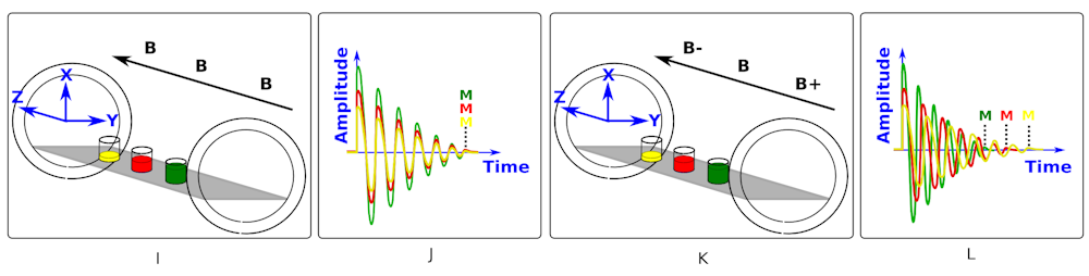
Figure I shows yellow, red and green glasses of water which represent the head, chest and abdomen of a patient in the scanner. We can see in figure I that the magnetic field - shown as B - is the same strength all along the z-axis. Figure J shows that after we “kick” the system, all three glasses of water respond by emitting radio waves of the same frequency. The signals have different amplitudes due to the different water levels.
Figures K and L show what happens if we make the field stronger at one end (B+) and weaker at the other (B-). We see in figure L that this gradient changes the Lamor frequency of the protons along the z-axis and the signals now have different frequencies.
So, by applying a magnetic field gradient and tailoring the frequency of the wave that “kicks” (excites) the protons we can select to only excite a thin slice of the patient.
Anyone who has had an MRI scan, will know that they are in the scanner for a significant length of time. This is because the patient has to be scanned slice-by-slice by applying the gradient and incrementing the frequency of the excitation. This is repeated many times to sequentially collect signals and build up an image from the slices of the patient.
While this discussion has brushed over a lot of the technical details, it serves to give a basic introduction to MRI and complements the articles on emission and transmission imaging.
Ideally (from ionising radiation considerations), all CT scans would be replaced with MRI. But, due to material differentiation, time and cost arguments these techniques must be used in unison.
Each of the techniques discussed in this series of articles - along with others than have not been covered, such as ultrasound - give clinicians a diagnostic arsenal to deploy when fighting our health problems.
Further reading:
SPECT and PET
X-rays and CT scans